Value Iteration

# Premise

Richard Bellman is one of the most legendary figures in computer science, having pioneered not only dynamic programming (DP), but also reinforcement learning.

The world can be thought of as a series of states, where each state has an associated value and different states are seperated by time. Consider a bouncing ball:

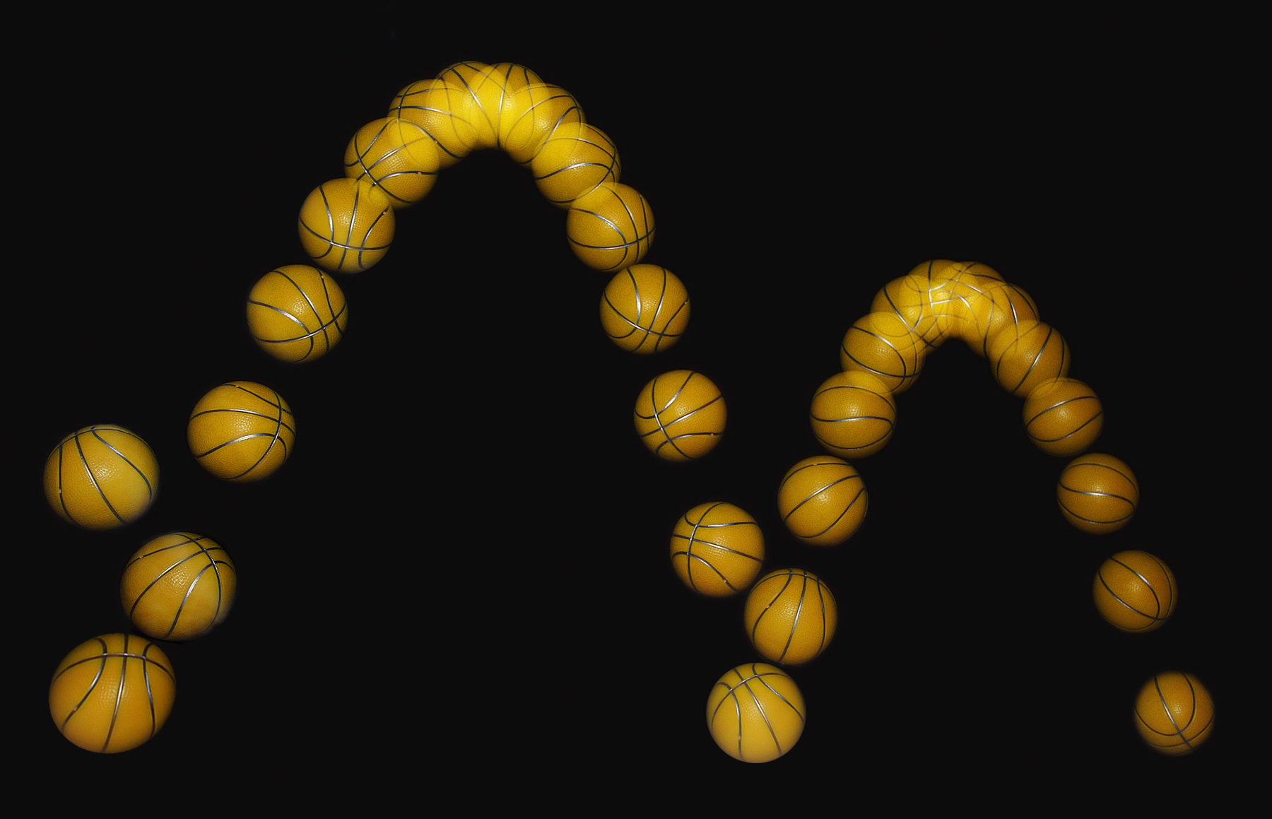Trajectory of Bouncing Ball From Michael Maggs

Each frame of the bouncing ball can be thought of as a state and each state can be associated with the value/utility, say the kinetic or potential energy of the ball. Each state is also seperated by time, in this case 1/25th of a second. The concept of states is central behind Markov decision processes (MDPs). MDPs are essentially networks where the states are nodes and the agent can take an action, which are represented as edges, to traverse to different states. In the example with the bouncing basketball, the agent would be the ball, and the action will be the ball falling/bouncing; in this example the agent cannot change its trajectory so the policy, or series of actions, is deterministic. The whole system of states and actions is called a Markov decision process (MDP); the ball decision does not involve any decisions so let's take a look at a more complicated example:

In this (simplified) example, the agent is Luke Skywalker on the planet Hoth riding a tauntaun escaping the stormtroopers. Luke starts on the upper left grid () and he is trying to reach the bottom right grid (). Luke on his tauntaun can chose from four actions in each state: move up the grid, move down the grid, move to the left on the grid, and move to the right on the grid. In other words, Luke and his tauntaun, as an agent, can make a decision on which action to take.

There are many obstacles along the way of Luke's journey, including grid which represents a wampa, which will most likely maul Luke to death. Luke will successfully escape the stormtroopers once he reaches but he will die if he reaches ; since the game ends when Luke reaches either or , they are known as terminal states. has a value of +1 since it's a desirable outcome (escaping the stormtroopers chasing him) while has a value of -1 since it's an undesirable outcome (getting mauled to death by a wampa). Furthermore, there is an insurmountable obstacle at , marked by X, Luke cannot enter that state. Since Luke is being chased, each move he makes increases the likelihood that the stormtroopers catch up; there is thus a penalty of -0.05 everytime Luke makes a move.

A visual way of visualizing a policy is to convert the gridworld into a graph; each cell would be a node, and there will be an edge between each pair of touching cells, such as and . A policy to traverse the gridworld is thus a path from the starting node to one of the terminal nodes, and . Looking at the grid, the optimal path is very obvious; there are two direct paths from the initial node to the terminal node (one going around over the obstacle and another going under the obstacle). Please note that the optimal path is as direct as possible, due to the negative penalty incurred with Luke deciding actions.

Why do we need value iteration if we can just solve the problem directly by tracing different paths?

For one, the grid can be much, much larger, and there can be many more obstacles and special conditions (for example, there can be traps set by stormtroopers which cause large penalties). It can thus be pretty difficult to trace and evaluate every individual path. Furthermore, the actions are often not deterministic; since Luke is riding a tauntaun, he doesn't have direct control over where the tauntaun decides to go. Luke may want to move left on the grid but the tauntaun may want to move down on the grid. For our example, let's assume that the tauntaun has an 80% chance of moving in Luke's desired direction and 10% chance of moving in the two perpendicular directions (for example, if Luke wants to go left, there is an 80% chance that the tauntaun moves left, a 10% chance that the tauntaun moves up, and a 10% chance that the tauntaun moves down).

It is clear that we should probably use a methodical way to approach this problem.

Here is where the ingenious value iteration dynamic programming algorithm comes in; the whole idea is to reduce the problem down to their simplest possible state and then solve the entire problem recursively.

# Intuition

The intuition behind Bellman's DP algorithm is to start at the terminal states (in our case and ) and trace the steps back to the starting state ().

Cracked Glass From WallpaperCave

Consider a glass cracked from one location; the cracks originate from one point and expand outwards, growing smaller the further it gets from the origin of the crack. The intuition behind Bellman's algorithm is to start at the origin of the crack (the terminal states) and work outwards. Then, if one wants to get to the desired terminal state, all one has to do is follow the cracks. Since the cracks get thicker the closer it gets to the terminal state, if for each move, we aim to get to a part on the glass where the crack is thicker, we can eventually trace back to the origin of the crack (terminal state).

# Algorithm

The value of the state (or intuitively the thickness of the crack) is defined by the Bellman equation as follows:

is the value of the current state, is the rewards/penalties received for the current state, and is the discounted reward for the optimal move into future state. is the discount rate and is the reward/penalty for taking action a from state s. We have a discount rate because we want to be able to control how much we value rewards in the future; if the rate is high (close to 1), it means that we value rewards in the future almost as much as we do in the future; if the rate is low (close to 0), it means that we do not value rewards in the future and only care about rewards at the current time. If is high, the algorithm will try to maximize the long-term success; if is low, the algorithm will try to maximize short-term gains. The is so that the optimal (reward-maximizing) step will be selected from state s.

FOr our example we will set our discount to 0.9.

The reward/penalty for taking action a from state s is defined as the sum of probability/reward pairs. For instance, for our example, if Luke wants to go left, there is an 80% chance that the tauntaun moves left, a 10% chance that the tauntaun moves up, and a 10% chance that the tauntaun moves down. is thus . If any of the directions are inaccessible, you move to the current state (if the agent wants to move down but cannot because of an obstacle or because of the boundary of the board, then we assume that the agent moves one step in place in the current grid).

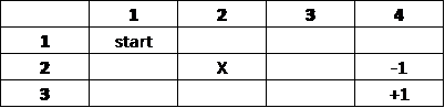
We will run Bellman's on our Star Wars gridworld.

Iteration 0:

Iteration 1:

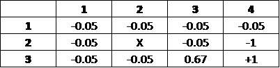
All but one of the accessible grids contained only the penalty (-0.05), since no surrounding grids from the previous iteration (Iteration 0) contained any values. The grid directly adjacent to the +1 terminal state has a value of 0.67; one can conceptualize Iteration 1 as making one move away from the terminal state. The calculation for the grid with value 0.67 () is as follows:

There are four actions which can be taken: going up, down (staying in the current grid), left, right (terminating the game). We will calculate the expected reward/penalty for each action:

It's important to note that since Luke is not guaranteed to go into the direction he choses, it's important to account for all possible directions which he can go. From the calculations, it's clear that the optimal move is to go right, as it has the largest expected reward.

We then plug this into the main Bellman equation:

In this case we have set our reward to be -0.05 (since taking actions causes time to pass which increases the chances of stormtroopers catching up) and our discount to 0.9 (0.9 is generally a good discount rate to start with).

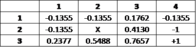
Iteration 2:

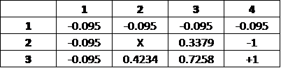
In Iteration 2, the two grids adjacent to the grid directly adjacent to the +1 terminal state has their values changed by more than just the penalty; one can conceptualize Iteration 2 as making 2 moves away from the terminal state.

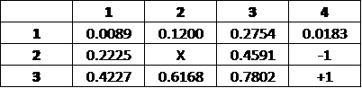
Iteration 3:

In Iteration 3, more grids are not only registering the penalty. This can be conceptualized as making 3 moves away from the terminal state.

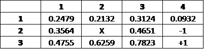
Iteration 5:

In Iteration 5, all of the grids have been affected by their neighbors; there are no longer any grids which are affected only by the penalty. From Iteration 5 on, the values change less each iteration and eventually converge. While we can technically run this algorithm as many iterations as we want, typically it's a good idea to have a threshold after which we assume the algorithm has converged; for example, if our theshold is 0.001, we stop the algorithm when the change in value for each grid is less than 0.001.

Iteration 13:

We halt the algorithm on Iteration 13. To find the optimal policy, we must once again apply the Bellman equation. Let's perform the calculations for :

Since moving downwards has the highest value, down is the optimal action for this state, and is thus a part of the optimal policy. We repeat this calculation for the rest of the states.

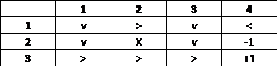
The optimal policy contains the best move to be made from each state/grid.

# Conclusion

Updating the different parameters of the problem, such as the amount of penalty that Luke receives for exploring, can affect the optimal policy. Please feel free to play around with the Excel file I used to write this blog; I have also written accompanying code in Python (also available on Github). Please feel free to experiment with different board configurations and different hyperameter values.

import numpy as np
import copy 

test = True

# initialize board (inaccessible states are represented with 'X')
grid = [[0, 0, 0, 0],
        [0, 'X', 0, -1],
		[0, 0, 0, 1]]

# specify goal states
goal_states = [(1,3),(2,3)]

# specify hyperparameters
discount = 0.9
R = -0.05
threshold = 0.001

# we're assuming that if a move is not deterministic, there is equal probability of 
# agent moving in the two perpendicular directions
# ie. if the action_probability is 0.8, if we choose to go left, there is 80%
# chance that we go left, 10% chance we go down, and 10% chance we go up
action_probability = 0.8

# outputs the current utility values of the board to stdout
def print_board(grid, it_num):

	print('ITERATION', it_num)
	len_x = len(grid)
	len_y = len(grid[0])
	for row in grid:
		for col in row:
			if col == 'X':
				print(col, end=" ") 
			else:
				print(round(col, 3), end=" ")
		print()
	print()

# checks whether the two grids are similar enough
def meets_criteria(grid1, grid2, threshold):
	len_y = len(grid)
	len_x = len(grid[0])
	
	for i in range(len_y):
		for j in range(len_x):

			if not (i == 1 and j == 1):
				if abs(grid1[i][j] - grid2[i][j]) > threshold:
					return False
	return True

# algorithm that iterates for optimal grid
def find_optimal_grid(grid, discount, R, threshold, goal_states, action_probability, print_intermediary):
	itnum = 0
	perpendicular_probability = (1.000-action_probability)/2.000
	# print_intermediary dictates whether the steps are printed
	if print_intermediary:
		print_board(grid, itnum)
	
	len_y = len(grid)
	len_x = len(grid[0])
	
	# find all inaccessible states
	inaccessible_states = []
	for i in range(len_y):
			for j in range(len_x):
				if grid[i][j] == 'X':
					inaccessible_states.append((i,j))
 
	while True:
		itnum += 1
		old_grid = copy.deepcopy(grid)
		
		# iterate through each cell in grid
		for i in range(len_y):
			for j in range(len_x):
				
				# check if cell is a terminal or inaccessible cell
				if (i,j) in goal_states or (i,j) in inaccessible_states:
					continue
				else:
					
					# iterative equations
					if (i-1,j) in inaccessible_states or (i-1 < 0):
						up_value = old_grid[i][j]
					else:
						up_value = old_grid[i-1][j]
					
					if (i+1,j) in inaccessible_states or (i+1 > 2):
						down_value = old_grid[i][j]
					else:
						down_value = old_grid[i+1][j]
					
					if (i,j+1) in inaccessible_states or (j+1 > 3):
						left_value = old_grid[i][j]
					else:
						left_value = old_grid[i][j+1]
					
					if (i,j-1) in inaccessible_states or (j-1 < 0):
						right_value = old_grid[i][j]
					else:
						right_value = old_grid[i][j-1]
					
					best = max((action_probability*up_value+perpendicular_probability*left_value+perpendicular_probability*right_value), 
								(action_probability*right_value+perpendicular_probability*up_value+perpendicular_probability*down_value), 
								(action_probability*down_value+perpendicular_probability*right_value+perpendicular_probability*left_value),
								(action_probability*left_value+perpendicular_probability*up_value+perpendicular_probability*down_value))

					grid[i][j] = discount * best + R
		if print_intermediary:
			print_board(grid, itnum)
		if meets_criteria(grid, old_grid, threshold):
			break
	
	# print optimal policy
	print('OPTIMAL POLICY')
	for i in range(len_y):
		for j in range(len_x):
			best_move = 'unset'
			best_move_value = float('-inf')

			if (i,j) in goal_states or (i,j) in inaccessible_states:
				pass
			else:
				best_move = []
				if (i==0) or (i-1,j) in inaccessible_states:
					up = grid[i][j]
				else:
					up = grid[i-1][j]
				
				if (i==2) or (i+1,j) in inaccessible_states:
					down = grid[i][j]
				else:
					down = grid[i+1][j]

				if (j==3) or (i,j+1) in inaccessible_states:
					right = grid[i][j]
				else:
					right = grid[i][j+1]
				
				if (j==0) or (i,j-1) in inaccessible_states:
					left = grid[i][j]
				else:
					left = grid[i][j-1]
			
				up_move = action_probability*up+perpendicular_probability*left+perpendicular_probability*right
				if up_move > best_move_value+0.001:
					best_move_value = up_move
					best_move = ['up']
				elif up_move >= best_move_value-0.001:
					best_move.append('up')

				down_move = action_probability*down+perpendicular_probability*left+perpendicular_probability*right
				if down_move > best_move_value+0.001:
					best_move_value = down_move
					best_move = ['down']
				elif down_move >= best_move_value-0.001:
					best_move.append('down')

				right_move = action_probability*right+perpendicular_probability*up+perpendicular_probability*down
				if right_move > best_move_value+0.001:
					best_move_value = right_move
					best_move = ['right']
				elif right_move >= best_move_value-0.001:
					best_move.append('right')

				left_move = action_probability*left+perpendicular_probability*up+perpendicular_probability*down
				if left_move > best_move_value+0.001:
					best_move_value = left_move
					best_move = ['left']
				elif left_move >= best_move_value-0.001:
					best_move.append('left')

			if best_move == 'unset':
				print(grid[i][j], end=' ')
			else:
				for k in range(len(best_move)):
					print(best_move[k], end=' ')
			print('|', end=' ')
		print()

if test:
	find_optimal_grid(grid, discount, R, threshold, goal_states, action_probability, True)